Reaction Diffusion in 3-Dimensions

latest Articles

Reaction Diffusion in 3-Dimensions

Articles —> Reaction Diffusion in 3-Dimensions

The Gray-Scott model is a mathematical model which describes behavior two chemicals based upon their diffusion, addition and removal rates, and reaction together. In an earlier article I described the details of the Gray-Scott Reaction Diffusion model. However this earlier description focused on the model in 2-dimensions. Taking this model a step further, here I describe how I modeled and visualized the Reaction diffusion model in three dimensions.

The Model in 3-Dimensions

In two dimensions a reaction diffusion model is represented by a 2-dimensional grid, visualization of which is via an image in which each grid value is represented by a pixel in the corresponding image. Creating a 3D implementation simply involves adding an additional dimension to the grid. However this additional dimension adds difficulties in computation, memory, and visualization, all of which are discussed below.

The mathematical model itself does not vastly change, but some aspects did require modification. For instance the diffusion operator - in 2D the laplacian operator - needed to be extrapolated to 3D. I experimented with several different methods, from a 3D laplacian kernel to an unbiased kernel in which every surrounding grid value is just as likely to diffuse (a center value of -1 and surrounding values 1/26), each of which can be another variable to play with.

Visualization

Visualization of the model is much more difficult in three dimensions. The results are a point cloud, each point containing a floating point value. To visualize this point cloud, I made use of an algorithm called marching cubes. Marching cubes¹ is a fascinating algorithm which helps find the convex hull of all points which are greater (or less than) a given value - here called the isolevel. In reaction diffusion terms, any concentration of A (or B) greater than a particular value is considered inside the hull. Marching cubes involves creating a grid of cubes, and for each cube within the 8 vertices represent adjacent isovalues of the 3-dimensional grid. For each cube the algorithm evaluates the vertices - some cubes are completely within or external to the hull, and can be skipped. However some cubes are found on the surface - a case in which the vertices of the cube are above and below the isolevel. In these instances marching cubes provides rules which determine where a triangle should be placed based upon which vertices are above and which are below the isolevel. More precise placement of the vertices of the triangle can be accomplished by linear interpolation of the isolevel along the edges where the triangle vertices reside. Marching cubes thus creates a list of triangles representing the surface, which can then be rendered in a 3D rendering engine - here I used OpenGL.

To nicely render each triangle using OpenGL shading the surface normals needed to be calculated. This calculation involved three calculations. First the normal at each vertex of a cube can be calculated- the normal being the gradient of the isovalue in the x, y, and z direction (more formally, this is simply the difference between isovalues of adjacent vertices). Next, the true normal of the point can be calculated by linear interpolation similar to that done for each point above. Lastly, some triangles share the same point in space, and the normals of all of these can be averaged out (either from the geometric mean, or a weighted average based upon the size of the triangle). While the surface normals I created in these images and movies below still need some perfection, they rendered fine for my needs.

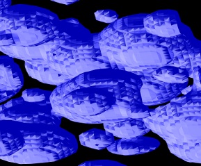
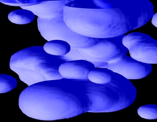
Left: No normal averaging. Right: Geometric Mean averaging of adjacent normals. Normals on the right could still use some work.

Finally, the process was set in motion. The grid was iteratively updated, the surface assembled with marching cubes, and the resulting surface rendered in OpenGL. To help in rendering, visualization, and analysis I added a few extra features such as model rotation, interaction dials to change parameters, and 2D slice images to visualize the model. Further, images of the model were saved an later compiled into movies using ffmpeg.

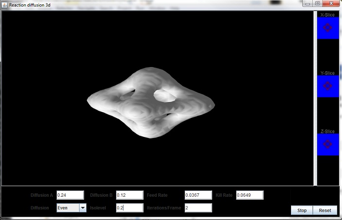
Reaction Diffusion OpenGL user Interface

3D OpenGL Reaction Diffusion User Interface (Java)

Difficulties

Some difficulties arose when constructing and analyzing the model:

Model Size: in 3-dimensions, the size of the model is cubic, thus the size of the model increases on a cubic basis. This forces one to use a large amount of RAM for any model of significant size, presuming one keeps the model in runtime memory. One could alternatively save the data to file and only load what is needed, for instance in a database, however I never took the analysis this far.
Iteration Time: The size of the model also increased iteration time. Every grid value needs to be calculated at each iteration, requiring at the very least O(x*y*z) time. Computation was sped up tremendously using OpenCL to place the work onto a GPU, however this affected parallel rendering using OpenGL.
The sweet spot: Different values of input variables (kill rate, feed rate, diffusion rate, etc...) yielded vastly different results. There exists a range of values within which dynamic shapes appear. In two dimensions one can create a map of values (see Robert Munafo's Reaction Diffusion Webpage) - these were difficult to map out in 3-dimensions. To aid in visualization, I created several images representing 2D slices, allowing me to visualize shapes of the 3D model in 2-dimensions.

Results

Once the programming had been complete I immediately found difficulty in hitting a sweet spot of parameters to create dynamic shapes within the model. I had played with different 3D kernels for diffusion, different diffusion constants, feed and kill rates, and different isolevels, all of which affected the model in vastly different ways. To help myself, I created a 3D grid with very shallow depth but large width and height. Across the x and y directions I increased the feed rate and removal rate, respectively. After seeding the grid this allowed me to nail down the regions of interest.