PCA For 3-dimensional Point Cloud
Articles —> PCA For 3-dimensional Point Cloud
Principal Component Analysis (PCA) is a technique to study the linear relationship of variables by converting a set of observations into a smaller set of (linearly uncorrelated) variables. PCA accomplishes this task by calculating the principle components of the data - sets of eigenvalues and eigenvectors of the covariance matrix of the data (an eigenvector is a non-zero vector which, when multiplied by a square matrix, yields a constant times the vector).
Multi-dimensional data can often be difficult to comprehend or even visualize - using PCA to reduce the data to smaller components can often be useful to summarize, or even extract meaning from, the data. Yet PCA itself can often be difficult to conceptualize, especially with multi-dimensional data. To better understand PCA, it can be easier by explaining in a smaller dimensional space (ideally one that can be visualized).
Consider a three dimensional point cloud in which the points are - in general - linearly correlated. The point cloud would thus fall along a plane in three dimensions. A point cloud such as this can be simulated in R using the equation for a plane...
a*x + b*y + c*z + d = 0
...where a = -0.1, b = 0.1, c = 1, and d = 0:
set.seed(1)#Set random seed value for reproduction

x = rnorm(100, sd = 1);#x values

y = rnorm(100, sd=0.5);

#Solve for z: z = -a*x - b*y - d

z = 0.1 * x - 0.1 * y + rnorm(100, sd=0.01) #0.2 * x + 0.3 * y + rnorm(100, sd=0.1);

xyz = data.frame(matrix(c(x,y,z), byrow=FALSE, ncol=3))

colnames(xyz) = c("x", "y", "z")

pairs(xyz, main="Point Cloud Pair Plot")
The above generates several random x and y points with a gaussian distribution around 0, and uses the equation of a plane to generate the z values. The standard deviation and plane values were chosen to constrain the 'spread' across each axis - the most variation along the x-axis and least along the z-axis (the reason for doing is for demonstration and will become evident later). The correlation of the values can be seen by plotting the values using the pairs function.
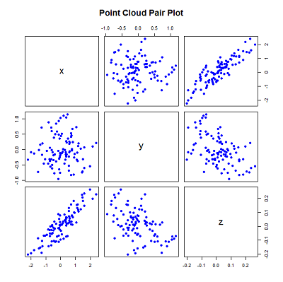
Pairs plot of simulated points in a plane. Note the x-y and - to a lesser extent - the y-z correlation.
One can also rely on 3-dimensional plotting using the rgl package in R:
library(rgl)

max = max(x, y, z);

plot3d(x,y,z,col="blue",type="s", radius=0.075, xlim=c(-max,max), ylim=c(-max, max), zlim=c(-max,max))

#Calculate the centroid and plot in a different color

centroid = c(mean(x), mean(y), mean(z))

spheres3d(centroid[1], centroid[2], centroid[3], radius=0.1, col="red")

#Render the plane

a = -0.1

b = 0.1

c = 1

d = 0;

#render the plane

planes3d(a,b,c,d, alpha=0.4)
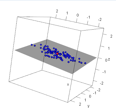
3-dimensional plot of points in R. Note the difference in variance along each axis.
Without diving into the math behind PCA, we can use the prcomp function in R to easily perform the analysis:
(pr = prcomp(xyz))

Standard deviations:

[1] 0.90272358 0.48134287 0.01022514


Rotation:

           PC1         PC2         PC3

x  0.994956814  0.01468438  0.09922352

y -0.004701295  0.99496568 -0.10010596

z  0.100193991 -0.09913463 -0.99001691
The resulting variable contains the eigenvectors (named rotation) and their associated eigenvalues (named sdev). Notice the eigenvectors are sorted by their eigenvalues largest to smallest - the first principle component (eigenvector) represents the most variance and the last component the least.
But what exactly do these values represent? First, let's see where these vectors point - the code below plots the eigevectors, each with their origin at the centroid of the data:
#render the eigenvectors - move so the vectors start at the centroid of the data

#First eigenvector

segments3d(c(centroid[1], centroid[1] + pr$rotation[1,1]), c(centroid[2], centroid[2] + pr$rotation[2,1]), c(centroid[3], centroid[3] + pr$rotation[3,1]), col="green", lwd=4);

#Second eigenvector

segments3d(c(centroid[1], centroid[1] + pr$rotation[1,2]), c(centroid[2], centroid[2] + pr$rotation[2,2]), c(centroid[3], centroid[3] + pr$rotation[3,2]), col="blue", lwd=4);

#Third eigenvector

segments3d(c(centroid[1], centroid[1] + pr$rotation[1,3]), c(centroid[2], centroid[2] + pr$rotation[2,3]), c(centroid[3], centroid[3] + pr$rotation[3,3]), col="red", lwd=4);
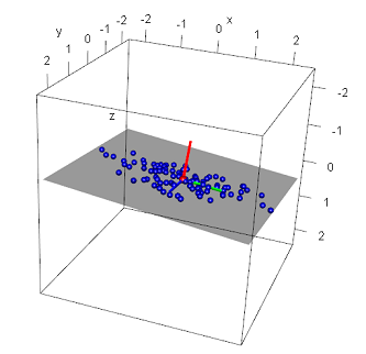
3-dimensional plot of eigenvectors. Note the first (green), second (blue) and last (red) eigenvectors.
Recall when generating these data points their 'spread' across each axis was constrained by using specific standard deviation and plane values: the x axis had the most deviation and the z-axis the least. When looking at the principal components, notice their direction: the first vector (green) points in the direction of the most variance (along the x-axis1), the second (blue) along the axis containing the second most variance (along the y-axis1), and the last (red) along the axis with the least amount of variance - along the z-axis1. By definition, this was to be expected. But also recall we used the equation of the plane to generate these points - note that the first two eigenvectors lie in this plane1. What about this last eigenvector? This vector lies perpendicular to the plane1. Also note the values of the third eigenvector: approximately equal to the plane values a, b, and c. In fact, a plane can be defined by its normal: the a, b, and c values in the plane equation being the x, y, and z values of the normal. Thus, given a set of points in 3-dimensions, the third eigenvector represents the surface normal of the regression plane of those points.
In higher dimensions, understanding and interpretation of these values becomes more difficult. However the principals hold true: the first eigenvector represents the direction of most variance, while the last represents the least. This is a useful concept, as one can rely on the first (or first several) eigenvectors from PCA (or vice-versa) for data analysis - useful in machine learning applications such as dimensionality reduction, clustering, and/or classification.
Links
1The eigenvectors lie approximately in the plane, as the randomness of the simulation results in noise.
Comments
- ASIF RASHA - January, 31, 2017
Thanks for the helpful tutorial. Just a question, if I want to rotate a transformed point cloud (xyz = -8.7 23.2 73.2) so it aligns with the centre (x,y,z)=0, how can I use the rotation from prcomp? I want to align the current xyz of the cloud (that I’m working with) to the xyz=0, and then transform it to the centre (which should be straightforward). Thank you!
- Richard Wert - July, 12, 2020
I am wondering you guys could put a demonstration of the Cloud systems would help alot