Programming the Lorenz Attractor
Articles —> Programming the Lorenz Attractor
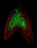
The Lorenz Attractor is a system of differential equations first studied by Ed N, Lorenz, the equations of which were derived from simple models of weather phenomena. The beauty of the Lorenz Attractor lies both in the mathematics and in the visualization of the model. Mathematically, the Lorenz Attractor is simple yet results in chaotic and emergent behavior. Visually, when the values given by the equations are plotted in two or three dimensional space the behavior is reminiscent of an orbit of an object around two central origins, when looked at from the appropriate dimension the pattern appears similar to a figure eight (see below).
There are three Lorenz equations that comprise the Lorenz Attractor, each of which can be though of as the x, y, or z component of a given three dimensional location in space:
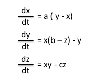
The Lorenz Equations.
Each of these equations can be read as the 'change in x,y, or z with respect to time'. Thus, each equation is used to calculate how much a given point is changed relative to the previous point, the change dependent upon the elapsed time.
The values a, b, c in the Lorenz equations are constants (for the Lorenz Attractor, a = 10, b = 28, and c = 8/3). These constants, as well as the above equations, can be altered to generate different results. For instance, a value of a = 1 results in a spiral with a single attractor (converging on this attractor), or a value of c = 20 results in a similar pattern given by c = 28, but with more compact orbits. Alternatively, other mathematical equations result in other types of attractors, such as the Henon Map or the Rossler Attractor.
The implementation of the Lorenz Attractor can be quite simplistic, as shown in the C source code below:
/*

* Basic Lorenz Attractor code

*/

double x = 0.1;

double y = 0;

double z = 0;

double a = 10.0;

double b = 28.0;

double c = 8.0 / 3.0;

double t = 0.01;

int lorenzIterationCount = 1000;

int i;

//Iterate and update x,y and z locations

//based upon the Lorenz equations

for ( i = 0; i < lorenzIterationCount; i++ ){

    double xt = x + t * a * (y - x);

    double yt = y + t * (x * (b - z) - y);

    double zt = z + t * (x * y - c * z);

    x = xt;

    y = yt;

    z = zt;

}
The code above simply loops lorenzIterationCount times, each iteration doing the math to generate the next x,y,z values (the attractor is seeded with values x = 0.1, y = 0, and z = 0). Note that time t is programmed in as 0.01, a relatively arbitrary (and seemingly unit-less) value that is multiplied by the differential equation to generate the change - or delta - in the x,y,z values.
A more comprehensive version written in Java is given below. The Lorenz class, along with the accessory Tuple3d class and Tranform interface (the former for 3-dimensional points and the latter to allow one to change the the mathematics of the attractor with a different implementation of the interface) can be used to iteratively generate the new points based upon the given equations (represented by the Transform implementation).
/**

 * Interface to transform an object T to a derived form of object T.

 * @author G Cope

 *

 */

public interface Transform<T> {


	/**

	 * Transforms and returns the transformation of the parameter val.

	 * @param val The object to transform

	 * @return The transformed object. Whether the returned value is the same or a different

	 *  	instance than val is implementation specific.

	 */

	public T transform(T val);

}


/**

 * Class to store 3-dimensional values.

 * @author G Cope

 *

 */

public class Tuple3d{


	public final double x;

	public final double y;

	public final double z;


	/**

	 * Constructs a new Tuple class.

	 * @param x

	 * @param y

	 * @param z

	 */

	public Tuple3d(double x, double y, double z){

		this.x = x;

		this.y = y;

		this.z = z;

	}


	@Override

	public String toString(){

		return "[" + x + ":" + y + ":" + z + "]";

	}

}


/**

 * Attractor based upon the Lorenz equations

 * @author G Cope

 *

 */

public class Lorenz{


	private Tuple3d current = new Tuple3d(0,0,0);


	private double a = 10d;

	private double b = 8/3d;

	private double c = 28d;


	private double dt = 0.1;


	/*

	 * The Lorenz equations implemented as a Transform of a Tuple

	 */

	private Transform<Tuple3d> transform = new Transform<Tuple3d>(){


		@Override

		public Tuple3d transform(Tuple3d val) {

			double dxdt = a*(val.y - val.x);

			double dydt = (val.x * (c - val.z) - val.y);

			double dzdt = (val.x*val.y - b * val.z);

			double nx = val.x + dt * dxdt;

			double ny = val.y + dt * dydt;

			double nz = val.z + dt * dzdt ;

			return new Tuple3d(nx, ny, nz);

		}


	};


	//Cumulative time.

	private double time = 0;


	/**

	 * Construct a new object with an initial point at the origin and time change of 0.1

	 */

	public Lorenz(){

		this(0,0,0);

	}


	/**

	 * Construct a new object with an initial point and default time change of 0.1

	 * @param x

	 * @param y

	 * @param z

	 */

	public Lorenz(double x, double y, double z){

		this(x, y, z, 0.1);

	}


	/**

	 * Constructs a new object with an initial point and change in time

	 * @param x

	 * @param y

	 * @param z

	 * @param time

	 */

	public Lorenz(double x, double y, double z, double deltaTime){

		current = new Tuple3d(x, y, z);

		this.dt = deltaTime;

	}


	public void setTransform(Transform<Tuple3d> transform){

		this.transform = transform;

	}


	/**

	 * Gets the current cumulative time.

	 * @return

	 */

	public double getCurrentTime(){

		return time;

	}


	/**

	 * Sets the delta time parameter

	 * @param dt

	 */

	public void setDt(double dt){

		this.dt = dt;

	}


	/**

	 * Iterates one step forward in time.

	 */

	public void iterate(){

		time += dt;

		current = transform.transform(current);

	}


	/**

	 * Retrieves the current location.

	 * @return

	 */

	public Tuple3d getCurrentLocation(){

		return current;

	}


}
To use the classes above, one can iteratively call the methods iterate() and getCurrentLocation, the former calculates the next point and the latter allows one to retrieve the new Point. Values from each iteration can be plotted in two or three dimensions - in java one has several options for visualization such as Swing or JOGL. A follow up article will dive into the details, with examples, for how to visualize and render the Lorenz Attractor.
There are no comments on this article.